Tips for Spatial Multi-Omics Experiments

At Aspect Analytics, we’ve been involved in numerous spatial biology projects. We’ve seen it all - seen a lot of good, and seen some…not so good. In this blog, we will share some of what we’ve learnt over the years with regards to wetlab decisions that can affect computational integration and downstream data analysis.  

We will focus on the following three things:

1. Spatial resolution of assays
2. How section selection for acquisition matters
3. Spatial feature size

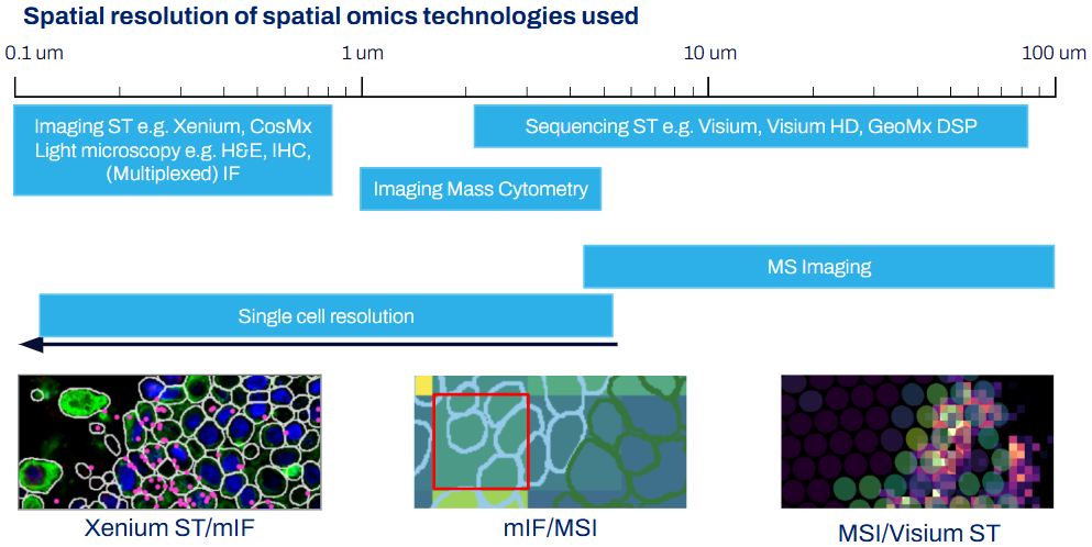
What is the spatial resolution of spatial biology assays? 

Right now it feels like there are so many spatial biology assays out there with new ones popping here and there. That’s true, but depending on your omics layer of interest, the spatial assays fall into clear categories. These categories then have quite clear spatial feature sizes. 

• Spatial Transcriptomics (ST) assays fall into two broad categories: Sequencing-based or Imaging-based [Williams CG et al, 2022]. 
  
  • For sequencing-based assays, transcripts are captured in an array or microdissected from regions of interest (ROI) and sequenced ex-situ. The spatial feature size therefore varies depending on the array or ROI size, typically ranging 2-100μm. Examples of this assay type include Visium and Visium HD, GeoMx or Stereo-seq.  
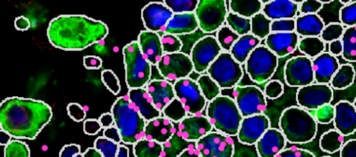
  • Imaging-based ST assays include CosMx, MERSCOPE and Xenium. Fluorophores are hybridised to transcripts and then imaged. The spatial feature size will therefore depend on the optics used - typically microscopy range of 0.1-1μm.
• Spatial Proteomics (SP) assays also fall broadly into imaging or mass spectrometry-based [Nature Methods, 2024].
  
  • Imaging-based SP uses antibodies tagged with fluorophores, e.g. COMET, PhenoCyclerFusion, have microscopy-level resolution
  • Mass spec-based assays can be further divided into microdissection or antibody-based 
    
    • Microdissection spatial proteomics uses laser capture microdissection to isolate ROIs and run ex-situ via LC-MS workflows. Resolution therefore varies depending on capture area. 
    • Antibody-based uses antibodies tagged with probes that are detected via mass spectrometry methods. The spatial feature size is 1μm for IMC and ranging from 5-50μm for MALDI-IHC
• Spatial lipidomics, metabolomics, glycomics and peptidomics. These assays are mass spectrometry imaging (MSI)-based assays, where commercially-available instruments have an upper resolution range of 5μm pixel size.  

So how does this affect data analysis? Put simply, use the assays that are appropriate for your scientific question. For example, if you want to profile changes in immune cell lipid content based on their distance from a tumor-stroma interface, you will need to have at least one assay that can allow you to profile individual immune cells and lipids at an appropriate gradient.   

What’s the difference between same, serial, consecutive or neighboring sections? 

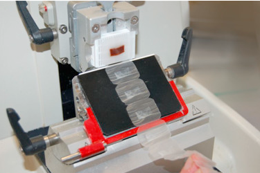
Spatial biology assays currently work by spatially mapping molecules across a tissue section. The section or sections from which the acquisitions are made also affects how you can integrate the data. Typically, histology labs cut tissues as ‘ribbons’, whereby sections come off together in a sequence, one after the other. 

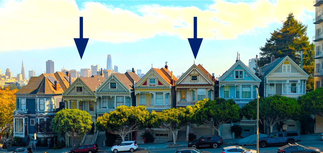
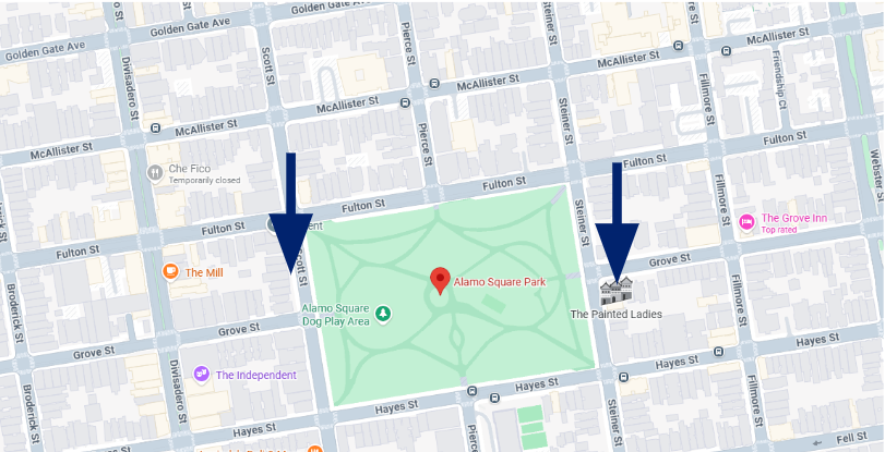
When every section that is cut is collected in sequence, e.g. collecting 10 sections in a row (no losses), these are serial sections. Why does this matter? To explain this, consider the Painted Ladies of Alamo Square in San Francisco:

If these houses were tissue sections, every house in this row can be considered as serial sections. 

Some spatial biology assays are compatible with sequential acquisition. This allows collecting data from the same section, for example spatial lipidomics, spatial glycomics, spatial proteomics and H&E one after the other, all from one section [V Denti et al. J Prot Res, 2022]. We can consider this analogous to different floor levels in the same house: 

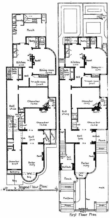
Same footprint, same location of walls, but different information being captured. Integration is fairly straightforward. The data has been acquired from exactly the same cells, so can integrate to the level of a single cell. 

However some assays are not compatible for sequential acquisition from a single section or maybe you decide you don’t want to acquire data from the same section (fair enough). In that case, you probably want to collect the data from consecutive (directly adjacent) sections e.g. section 1 and 2 from a serial cut. 

While you are unlikely to be in the same cell (depending on section thickness), you can be confident that the cell populations are similar. For integrating data from consecutive sections, it is therefore possible to integrate to the level of cell populations, multi-cellular environments, or defined spatial footprint. 

Where things get tricky is the idea of neighboring sections. Ideally “neighboring” sections mean the same as “consecutive” sections. However, the house a few doors down is also a neighbor, the same way the house down the block in the same area code can also be considered a neighbor. 

Likewise, neighboring sections can be section 1 and 4 from a serial cut. And continuing the house analogy, houses a few doors down or across the block probably don’t have the same floorplan but it probably does have similar features. In this case, for neighboring section acquisitions, data can be integrated to the level of structures or anatomical regions. 

And then finally there are ‘neighboring?’ tissue sections. These are tissue sections from the same block, but where it’s very hard to find any matching characteristics between the sections. We sometimes see this when the tissues get acquired by someone not closely involved in the actual experiment, often meaning well to get the best sections, but in doing so removing a significant number of adjacent sections. Integration is usually more of a ‘best’ effort scenario at that point, and requires a different way of integrating the data altogether. If possible, try to avoid this, as it limits the scope of analysis and makes us sad.

In short:

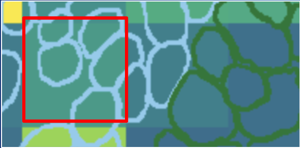
How does spatial feature size affect computational integration? 

The size of the target feature of interest compared to the spatial resolution of the assay used for acquisition naturally plays an important role in the downstream analysis. In an ideal setting we have (i) pixel or spot sizes that are (significantly) smaller than the target feature size, and (ii) multiple pixels in the target feature. This allows us to (i) spatially distinguish it from its surroundings and (ii) provides multiple measurements for the spatial feature, which increases confidence in the observed signal.

• Is your feature big or small?
  
  • Big? Can use larger spat res assays across different sections
  • Small? Try to use smaller spat res assays from same or consecutive sections as possible
• Understand the scientific assumptions you are making with integration and if you’re okay with them 
  
  • e.g. wanting to integrate to single cell level when acquisitions are from neighboring sections or not acquired at single-cell or close to single-cell resolution assays.  
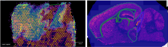
• Say you are doing neuroscience research and interested in the transcriptomic and lipid profiles of brain structures. Unless you are interested in very specific features or cell populations, you don’t have to use the highest resolution assays. However, if your question is more specific, such as if the transcript and lipid profile of microglia (small cells) varies on their distance from the third ventricle (large feature), it will be more difficult to assign signals to specific cells if the data is acquired at too low a resolution.

Conclusion

Maximising spatial multi-omics insights requires careful consideration at three levels. First, choose assays whose spatial resolution matches your biological question — single-cell queries demand high-resolution platforms. Second, plan your section strategy deliberately: same-section acquisitions enable single-cell integration, consecutive sections support cell-population-level analysis, while neighboring sections limit you to structural or anatomical integration. Finally, ensure your target feature size aligns with assay resolution. Getting these decisions right before acquisition saves significant analytical headaches downstream and ultimately determines the depth of biological insight you can reliably extract from your experiment. 

TL:DR

Maximising spatial multi-omics insights comes down to three pre-acquisition decisions. 

1. Match your assay's spatial resolution to your biological question. Imaging-based assays reach ~0.1–1μm (single-cell), while sequencing-based arrays and mass spec acquisitions typically range 2–100μm. 
2. Plan your section strategy: same-section acquisitions enable single-cell integration, consecutive (directly adjacent) sections support cell-population-level analysis, while neighboring sections (with gaps between them) limit you to structural or anatomical-region integration. 
3. Ensure your target feature is large enough relative to your assay resolution to be spatially distinguished and measured with confidence. 

Get these three things right before you cut your first section, and the downstream analysis becomes significantly more tractable.

‍

This blog is based on Nico Verbeeck's presentation at the ASMS 2026 MS Imaging workshop.