Introduction to mass spectrometry imaging data analysis

This post is part of our series titled "Mass spectrometry data introduction", which contains the following entries:
- Introduction to mass spectrometry data analysis
- Introduction to mass spectrometry imaging data analysis (current post)
Table of contents
Introduction
Mass spectrometry imaging is a molecular imaging modality that can map the spatial distribution of a large number of molecules in a biological tissue section, with an unparallelled chemical specificity. MSI does not require prior tagging of molecular targets and is able to measure a large number of ions concurrently in a single experiment. Many of these advantages are due to the fact that, as the name suggests, MSI data is acquired through use of a mass spectrometer. The result data is sometimes referred to as a hyperspectral image cube, a basic illustration of which is shown in Figure 1.
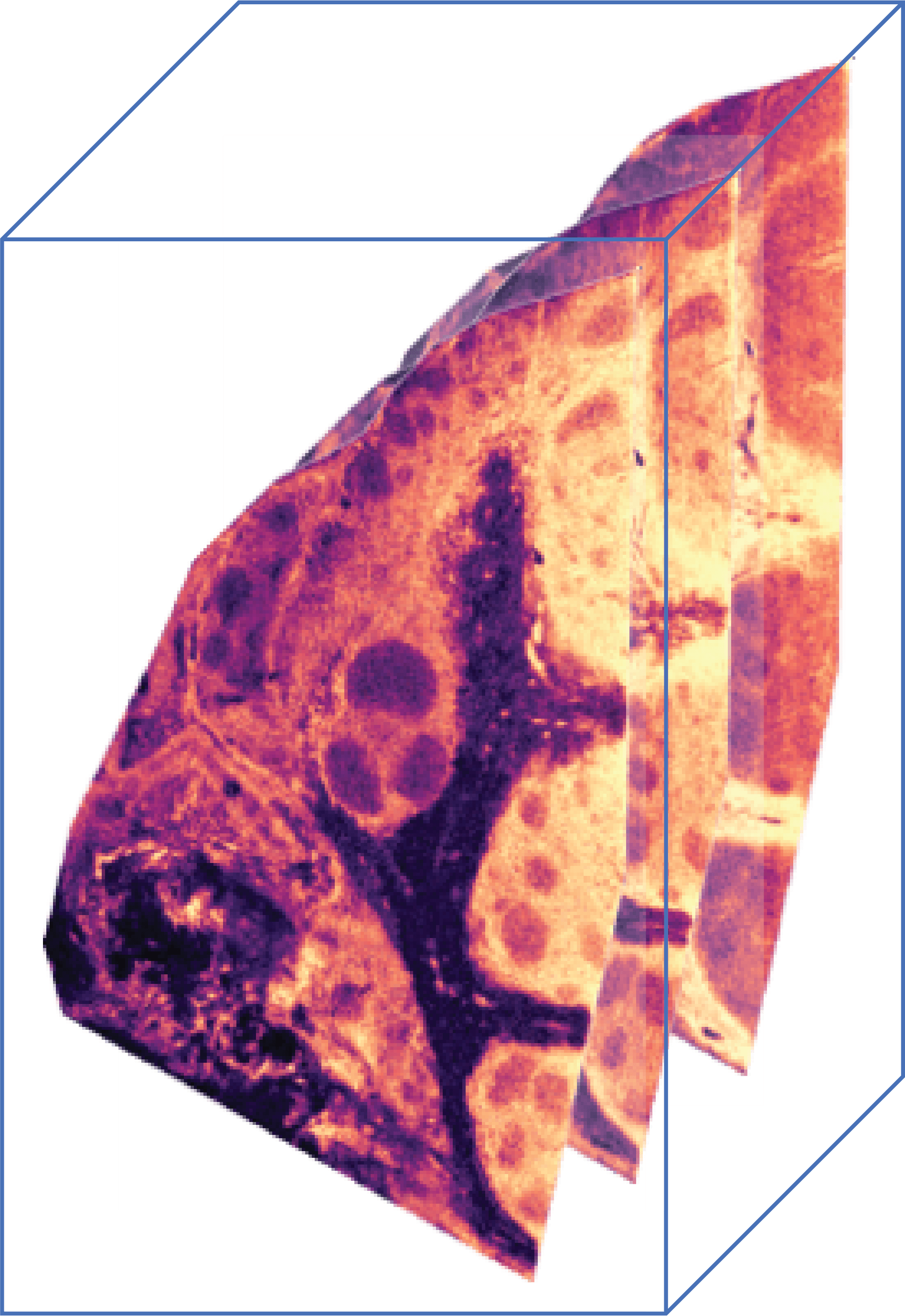
Similar to how a typical camera makes an image with three color channels, namely red, green and blue, where each channel represents the intensity of specific wave length of light, MSI generates images that can have tens of thousands to over a million of different “channels”, where each channel represents the intensity of a specific m/z value (mass over charge).
Owing to its roots in MS, MSI similarly enables untargeted screening of thousands of biomolecules in a single experiment, i.e., in one tissue section. Additionally, using MSI we can investigate the localisation of various molecular classes, including proteins, peptides, lipids and metabolites, some of which are not readily accessible using other approaches. Due to all of these properties, MSI is a phenomenal platform for life sciences research.
However, the technology generates large, complex datasets and thus emphasizes the importance of data analysis. At the time of writing, a single experiment - i.e., one tissue section - typically yields tens of gigabytes up to multiple terabytes of raw data. As such, efficient, streamlined bioinformatics workflows are necessary to process the resulting data and extract the maximum amount of insight in a timely manner, especially in high-throughput settings. Fortunately, you’ve come to the right place for that!
Mass spectrometry imaging (MSI) data acquisition
A MSI experiment involves acquiring mass spectra at various locations (pixels) in a tissue section. Conceptually, an MSI data set is an image where each pixel has an associated mass spectrum. An example of a typical MALDI MSI experiment is shown in the animation below.
Briefly, a tissue section is cut about 8-10 micrometers thick, and mounted onto a glass ITO slide. The tissue is then covered with a chemical matrix, which assists in ionization process, and is then put in the mass spectrometer. Then, a virtual grid is laid out, and subsequently a laser is fired in each cell of this grid. This ionizes the molecules in that location, and those locally generated ions are then sent to the mass analyzer to obtain a mass spectrum is collected for that pixel. This processes is repeated for each grid cell. While other methods of ionization operate slightly differently, the overall concept of local ionization remains comparable.
The animation illustrates the key steps in a MALDI MSI experiment. First, the tissue is coated using a chemical matrix which assists in the subsequent ionization process. Firing the laser in each grid cell ionizes the tissue locally, enabling us to obtain a mass spectrum with localized chemical information from the resulting ions. This procedure is repeated in every cell of the grid.
MSI instruments generally differ from non-imaging MS instruments in the fact that they have a fast-moving stage and a laser with a high firing rate to enable acquiring spectra at different locations on the section at a greater speeds. This is especially true for instruments aimed at acquiring MSI data with high spatial resolution, which results in a lot of pixels being acquired. In general, in order to keep measurement times feasible, a trade-off will be made between a lower number of pixels measured at a high mass resolution (low spatial resolution, long measurement times per pixel), or a high number of pixels at a low mass resolution (high spatial resolution, low measurement time per pixel).
The MS instrument itself - apart from the source - usually operates in the same way as in non-imaging MS. Most modern instruments used for MSI are designed specifically for imaging, though some non-imaging MS instruments are commonly made imaging-capable using custom sources.
Since MSI is based on mass spectrometry, most advantages and challenges from MS naturally map onto MSI. That said, it is important to be aware that some tricks that are used in other forms of MS can not be used in the context of imaging, for instance physical separation of certain components within a mixture using liquid chromatography. Bluntly speaking, in MSI we usually end up analyzing the soup of cells in the way it is served in the tissue, with few ways to filter out components we’re not interested in during the experiment.
MSI data
As mentioned in the introduction, MSI data sets can be interpreted as spectral images, in which each pixel is associated to a mass spectrum. A standard MSI data set has three key axes, the spatial axes (x and y) and the spectral axis (m/z). Some more advanced approaches like ion mobility can add additional axes to the data, but we will not discuss those here.
At the time of writing, pixel counts tend to vary from a couple thousand up to over a million per tissue section, whereas the amount of m/z bins can similarly vary between a couple thousand to several million per spectrum. In the particular case of SIMS, which boasts extremely high spatial resolution, the number of pixels can be an order of magnitude higher.
Raw data size is directly related to the amount of pixels in the data set and the number of m/z bins per spectrum. Let’s assume an example MSI data set comprising around 50.000 pixels and 100.000 m/z bins per spectrum. When storing the intensity data as 32-bit floating point numbers, as is commonly done, a data set of this size will amount to about 20 GB of storage. If we assume a 50 micrometer spatial resolution, 50.000 pixels roughly correspond to an imaged surface area of 125 mm2, e.g., a square with edges of about 1.12 cm.
Matrix representation of MSI data
When representing MSI data in matrix form, D∈Rm×n is a data matrix where rows denote pixels and columns denote m/z bins. Hence, for a single MSI data set, m is the number of pixels and n is the number of spectral bins or m/z bins, i.e. each row of D represents the mass spectrum of a pixel in the sample along a common m/z binning.
This matrix representation of MSI data does not directly encode the spatial localisation of the individual pixels (rows), but for many types of data analysis - both supervised and unsupervised - these locations are not required. In practice, the specific grid coordinates of each spectrum are of course retained as well in a separate data structure.
When we consider high spatial resolution experiments, the data matrix is usually tall (many pixels, relatively few m/z bins), whereas high mass resolution experiments tend to give rise to wide data matrices (fewer pixels, many m/z bins). Depending on the type of data analysis, the shape of the data matrix may have a profound impact on computation time and memory requirements.
The matrix representation of MSI data mandates that all spectra are encoded using the same m/z bins (columns of D), which may require explicit realignment during data analysis. In MSI lingo, data sets in which all spectra share a common set of m/z bins are sometimes referred to as being in continuous format, based on the nomenclature used in the imzML data format.
Example use cases
In this section we will show some of the basic ways of analysing MSI data. MSI data can be sliced along the m/z axis, giving rise to images showing the localisation of biomolecules, and spatially by extracting spectra from a certain region of interest. In practice, most data analysis pipelines combine these complementary and mutually synergistic data analysis strategies. We will show an example of both in this section.
In these illustrations, we will use a MSI dataset acquired in human lymphoma tissue using a Bruker rapifleX MALDI Tissuetyper instrument. The experiments focused on lipids with 2,5-DHB matrix deposited by sublimation. A sampling resolution of 10 microm was used, collecting around 500.000 pixels. We focus on the m/z range of ~600-1000 Da resulting in 6000 ion images.
Ion images: visualizing spatial localisation of biomolecules
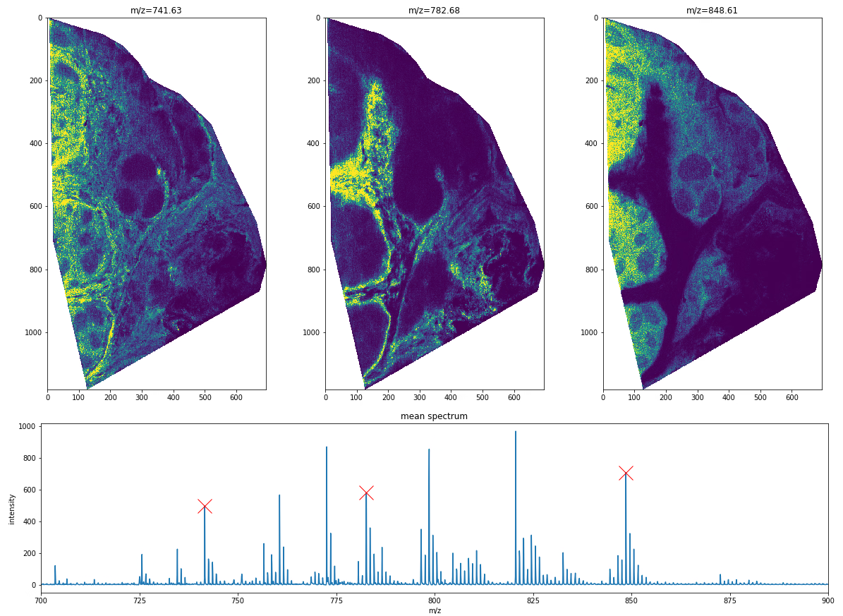
MSI data enables us to visualize the spatial distribution of biomolecular ions with a specific mass-to-charge ratio (m/z value), by plotting the intensities for that m/z value across all pixels. In MSI terminology, the resulting visualization is called an ion image. Essentially, an ion image displays a heat map rendered using a color map of choice. Since these colors are not truly observed, they are sometimes called false color images. Figure 3 below depicts three example ion images at different m/z values.
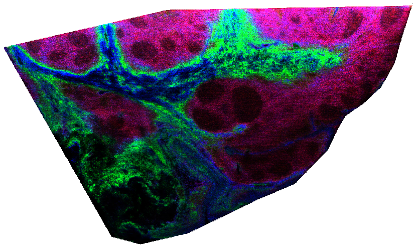
One of the key advantages of MSI technology is that we can investigate the localisation of thousands of biomolecular ions simultaneously, whereas most other technologies are usually limited to only a handful or a couple hundred at best. Naturally, the spatial distributions of various biomolecular ions can be multiplexed onto a single image in various ways. The simplest approach is to assign color channels to different m/z values, as shown below. For more complex ways of joint visualization we refer to subsequent blog posts.
Region of interest (ROI) analysis
This use-case is complementary to the one shown above. Here, we will exploit MSI’s spatial information to mark two regions of interest and investigate the biomolecular composition of those regions. This is a key differentiator between MSI and non-imaging MS technology.
In practice, regions of interest could be defined based on many properties, for instance tumor versus healthy tissue, anatomical structures within the tissue, specific cell types or even based on the localisation of certain marker ions within the MSI data. Very often, MSI data is paired with a stained microscopy section (usually H&E), which could then also be used to identify regions of interest based on morphology. Regardless of how they are defined, note that these regions are independent from the MSI data acquisition process, i.e., they can be defined during post-acquisition data analysis.
In Figure 5 below we’ve annotated two regions of interest on the ion image, shown in red and blue. A common use-case would be to compare the chemical content of those two regions.

In Figure 6, we’ve visualized the mean spectrum for each of these regions and it is immediately apparent that significant differences exist on a chemical level. In this example we’ve just computed the mean spectrum per region. In real use-cases, one might want to build classification models to distinguish these regions based on chemical information, or determine which biomolecules are differentially expressed between these regions, etc.

If we would have analyzed this tissue using non-imaging MS, the first step would have been to homogenize the tissue. The resulting single mass spectrum would essentially be a convoluted mixture of the spectra of all chemically distinct regions that make up this tissue. Hence, a key strength of MSI technology is that it enables us to select MS spectra from homogenous regions within tissue, for instance within anatomical structures rather than a full organ. This opens up significant potential to identify differences on a molecular level in small regions of tissue, for which the signal would be easily overlooked using non-imaging MS.
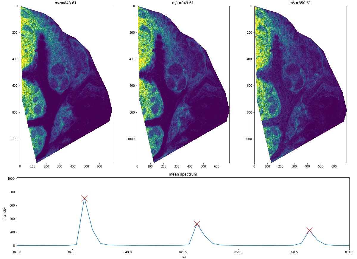
Detecting isotopes
In this final example we’ll show that MSI data is very powerful to detect isotopes. In non-imaging MS, one has to rely on assessing whether a series of peaks corresponds to an expected isotopic distribution with some statistical certainty.
With MSI, we can additionally use the corresponding ion images for all potentially relevant peaks to check consistency in spatial expression. If we are indeed looking at isotopes, the spatial expression should be close to identical, as these molecules have the same biochemical behaviour in the tissue.
Figure 7 shows an example of three isotopic peaks and their corresponding ion images. Based on the spectra, we can see that these peaks are roughly 1 Da apart, and thus likely to be isotopic peaks. The ion images further reveal that the spatial expressions of these peaks are near identical, which further adds to the likelihood that these are indeed isotopes. Of course the higher the mass resolution of the mass spectrometer, the more confident one can be in this assessment, and ultimately, identification would be necessary to unravel the nature of the analyte, which goes beyond the scope of this introduction.
Conclusion
In this post we’ve provided a birds-eye overview of mass spectrometry imaging. We’ve discussed the technology’s data acquisition workflows along with key properties of the resulting data and showed some example use-cases to illustrate MSI’s potential.
If you have any questions or suggestions related to the content of this post, please contact us!